0. Introduction

Learning math can be hard for several reasons, but one of them is that the language used by authors tends to be optimized for specialists:

• symbols and identifiers are heavily overloaded
• math writers abhor boilerplate
• a lot of the context of a given expression is assumed to be available to the reader, etc.

In addition to that, most math is written on plain paper or paper-like mediums such as PDF.

(If you look at this practice from the perspective of a programmer this is a bit strange: it's as if programs were written primarily using the plain text editor "Notepad", and without any help from the type checker)

But probably the main difficulty is just abstraction itself. One can spend a lot of time trying to come up with a good mental representation of new concepts.

As it turns out, we can use Scala (or other programming languages) to encode many mathematical definitions and ideas, and get some immediate wins:

• The typechecker can point out many errors.
• We get access to all the tools available when using a modern IDE, such as code completion, navigate to definition, inline documentation, auto-generated code, etc.
• A lot of the ambiguity is removed since we're forced to write every single definition in painful detail.

And crucially, we can re-use our existing programming intuition to help develop a purely abstract math intuition.

Of course we'll have to make some compromises in generality, but the reality is that most people don't learn (or do) math at the maximum possible level of generality (in part because that level is not fixed: it normally increases over time). All this is to say that for the ideas that can be expressed in our programming language, we are doing real math.

Now while Scala can be used to automate some theorem proofs (a topic for a different post), it is not a theorem prover such as Lean, or Agda. If you're seriously interested in doing math on your computer at the maximum generality then a proof assistant (an interactive theorem prover) is the best tool.

In this article we'll explore how we can encode several definitions from the book Category Theory and Applications by Marco Grandis and translate them into Scala 3.

Quoted text like this will be reserved for quotes from this book.

We'll end up by stating and proving the Yoneda lemma and explaining the (in)famous phrase "Monads are just monoids in the category of endofunctors".

Note 1: This article focuses mostly on the process of encoding Algebraic concepts into Scala, and is not meant to be a full tutorial on Categories.

Note 2: If you're not familiar with type functions then I recommend perusing Illustrated guide to Types, Sets and Values.

Note 3: All the code of this post is one Scala file. If you put the blocks into different files, two things fail. A companion object (for example object Functor) must be in the same file as its trait. And import zio.prelude.* also imports zio.prelude.Id, which then hides our type Id[A] = A.

Audience: Math beginner-ish, Scala intermediate.

Scala 3 version used: 3.9.0

Updated code available at: https://github.com/jpablo/math-with-scala

1. Categories

Informally, a category is a special kind of directed graph with an operation similar to path concatenation defined on the edges.

A Category $C$ consists of the following data:

1. a set $O$ whose elements are called objects of $C$.

2. for every pair $(X,Y)$ of objects, a set $\mathrm{Hom}(X,Y)$ (called a hom-set), whose elements are called morphisms (or maps, or arrows) of $C$ from $X$ to $Y$ and denoted as $f: X \rightarrow Y$,

The set $\mathrm{Hom}(X, Y)$ is also written as $C(X, Y)$

3. for every triple $X, Y, Z$ of objects of $C$, a mapping or composition

$$\begin{matrix} \mathrm{Hom}(X, Y) \times \mathrm{Hom}(Y,Z) & \rightarrow & \mathrm{Hom}(X, Z) \\ (f, g) & \mapsto & g \circ f \end{matrix}$$

These data must satisfy the following axioms

1. Associativity. Given three consecutive arrows $f:X \to Y$, $g:Y \to Z$, and $h:Z \to W$, the equation $h \circ (g \circ f)=(h \circ g) \circ f$ holds,

2. Identities. Given an object $X$, there exists an endomorphism $e: X \to X$ which acts as an identity whenever composition makes sense; in other words if $f: X' \to X$ and $g:X \to X''$, one has $e \circ f = f$ and $g \circ e = g$.

$e$ is called the identity of $X$ and written as $1_X$ or $\mathrm{id}X$.

1.1 Categories over the set of all types 𝕋

Our approach will be to represent objects as types (i.e. elements of the set $\mathbb{T}$ of all types), and hom-sets as type functions $\mathbb{T} \times \mathbb{T} \to \mathbb{T}$.

trait Category[Hom[_, _]]:
  type ~>[A, B] = Hom[A, B]
  
  extension [A, B, C] (g: B ~> C)
    def ◦ (f: A ~> B): A ~> C

  extension [A, B, C] (f: A ~> B)
    def >>> (g: B ~> C): A ~> C = g ◦ f
  
  def id[A]: A ~> A

  @Law
  def associativity[A, B, C, D](
    f: A ~> B,
    g: B ~> C,
    h: C ~> D
  ) =
    h ◦ (g ◦ f) <-> (h ◦ g) ◦ f

  @Law
  def identityR[A, B](f: A ~> B) = f ◦ id[A] <-> f
  
  @Law
  def identityL[A, B](f: A ~> B) = id[B] ◦ f <-> f

Laws are usually expressed as functions that return an instance of the case class IsEq(lhs, rhs), (the operator <-> is provided by Cats, it simply creates a new IsEq), which is then used in conjunction with the library discipline and ScalaCheck to generate random values and try to find counterexamples.

In this post, @Law is a marker annotation: case class Law(description: String = "") extends scala.annotation.StaticAnnotation. Our <-> is stricter than the <-> of Cats: it compiles only when the two sides have the same type (extension [A](lhs: A) def <->[B](rhs: B)(using ev: B =:= A): IsEq[A] = IsEq(lhs, ev(rhs))).

(Here's the updated code of these definitions, in the repository of this post)

Some of the types involved in this definition are:

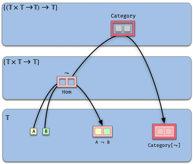
with composition:

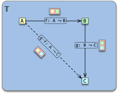
Notation can get heavy pretty fast, so the arrow notation A ~> B is very convenient as long as we remember that arrows are not necessarily functions (and as a reminder of this I decided to use Hom[_, _] for the parameter name).

In particular notice that there's no evaluation function defined on arrows, which means that everything needs to be done "point-free" when using the Category trait.

Example: Pure Scala functions and types

Probably one of the most elementary categories in math is the Set category of sets and functions.

Arguably the Scala category (with types as objects and pure functions as arrows) defined below plays a similar role, in the sense that it is the "base" language on top of which everything else is built.

type Scala[A, B] = A => B

given Scala: Category[Scala]:
  def id[A]: A => A = identity[A]
  extension [A, B, C] 
    (g: B => C) def ◦ (f: A => B) = g compose f


// This satisfies the category laws but 
// only for pure functions :)

From now on we'll refer to this category simply as Scala.

(Scala 3 feature: given instances).

Implicit or explicit?

There's no requirement to make the Scala category instance an implicit value (I mean... given). But in most cases we'll be using only one category instance C for a given hom function Hom[_,_]. In this situation it's very convenient to be able to just pass the hom function and have the corresponding category instance be looked up by the compiler (and we can always use an explicit instance when needed).

Here's a summary of how we translated the definition into Scala:

The textbook definition allows for the objects $O$ of the category $C$ to be an arbitrary set, whereas in our Category trait we have no way to restrict the arguments for Hom, which means that instances of this trait have a fixed set of objects O: the set of all types!

In order to create more general categories we need to find a way to restrict objects to be members of different sets of types.

There are two main ways in which we can specify subsets of types in Scala:

1. Via subtyping
2. Via type classes

Long story short, we'll have to create slightly different Category definitions to express different kinds of constraints over the arguments of Hom. We'll use our original definition when possible though, because other definitions add some boilerplate.

Type arguments vs type members

Another encoding choice would be to use an abstract type member like so:

trait Category:
  type Hom[A, B]
  def id[A]: Hom[A, A] 
  extension [A, B, C] (g: Hom[B, C]) def ◦ (f: Hom[A, B]): Hom[A, C]

I find this approach more cumbersome to deal with, mainly due to the fact that it can be easy to get the types wrong, and harder to fix. Also you end up having to use things like the Aux[_] pattern frequently to reduce boilerplate and prevent errors.

Example: Category of types and subtyping relationships

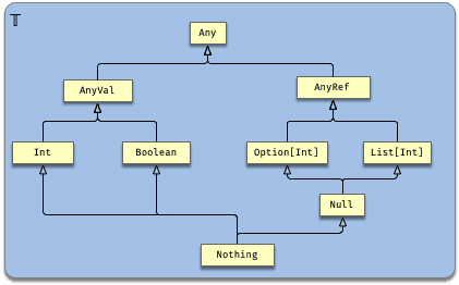
We know that types in Scala form a lattice under subtyping:

A natural category to consider would be one with all types as objects and a single morphism between A and B if A <: B (and no morphisms otherwise).

(This is called the Liskov category in Scalaz)

Scala provides a data type (<:<[A, B]) that encodes the fact that type A is a subtype of B

given Subtypes: Category[<:<]:
  def id[A] = <:<.refl
  extension [A, B, C] 
    (g: B <:< C) def ◦ (f: A <:< B): A <:< C = 
      g compose f

For each pair of types A <: B there is only one arrow, the unique value of type A <:< B that can be obtained using summon (and none otherwise):

trait A
trait B extends A
trait C extends B

Subtypes.id[A] == summon[A <:< A]

import Subtypes.~>

val f: C ~> B = summon[C <:< B]
val g: B ~> A = summon[B <:< A]
val h: C ~> A = summon[C <:< A]

g ◦ f == h

Example: Product category

If $C$ and $D$ are categories, one defines the product category $C \times D$.

An object is a pair $(X, Y)$ where $X \in C$ and $Y \in D$. A morphism is a pair of morphisms

$$(f, g): (X, Y) \to (X', Y')$$

for $f\in C(X, X')$ and $g \in D(Y, Y')$.

Thus for us objects will be types of the form (A, B) and arrows tuples of arrows (C[A1, A2], D[B1, B2]).

First we use match types to define two functions that can only be applied to types of tuples, and can extract the first and second arguments (i.e. the first or second type):

type _1[X] = X match { 
  case (a, _) => a 
}

type _2[X] = X match { 
  case (_, b) => b 
}

Morphisms are tuples of morphisms:

type ×[~>[_, _], ->[_, _]] = [A, B] =>>
  ( _1[A] ~> _1[B],
    _2[A] -> _2[B] )

The operator × constructs the product category:

// C × D
extension [C[_, _], D[_, _]]
  (C: Category[C]) def × (D: Category[D]): Category[C × D] =
  import C.◦ as ++
  import D.◦ as +

  new Category[C × D]:
    def id[A]: A ~> A =
      ( C.id[_1[A]],
        D.id[_2[A]] )

    extension [A, B, C] 
      (g: B ~> C) def ◦ (f: A ~> B): A ~> C =
      ( g._1 ++ f._1,
        g._2 +  f._2 )

Example:

val Scala2 = Scala × Scala

val (f, g) = Scala2.id[(Int, Char)]
// f == identity[Int]
// g == identity[Char]

1.2 Other encodings

Example: Monoids as a category

As an example of a category where the arrows are not functions, consider a category with only one (arbitrary) object * and whose morphisms are the natural numbers $0, 1, 2, \dots$. The composition of two morphisms is their sum, and the identity is $0$.

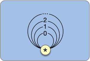
The previous Category definition won't work here because the Hom function accepts arguments of any type.

One way to restrict the arguments is to add a common upper bound everywhere:

trait CategoryS[U, Hom[_ <: U, _ <: U]]:
  type ~> = Hom
  def id[A <: U]: A ~> A
  extension [A <: U, B <: U, C <: U] (g: B ~> C) def ◦ (f: A ~> B): A ~> C

// Category laws modified accordingly

Now we can choose an arbitrary value (say the String "Singleton") and use its singleton type as the upper bound U:

// The singleton type of the String "Singleton".
// Any other singleton type will work.
// Strictly, the objects are all the types A <: ●,
// for example ● itself and Nothing. But every hom-set
// is ℕ, so all these objects are isomorphic, and
// the category is equivalent to a one-object category.
type ● = "Singleton"
type ConstantHom[A] = [_ <: ●, _ <: ●] =>> A

// The natural numbers 0, 1, 2, … under addition.
// BigInt has no maximum, so a sum never overflows.
case class ℕ(n: BigInt):
  require(n >= 0, s"$n is not a natural number")
  def + (m: ℕ): ℕ = ℕ(n + m.n)

object ℕCategory extends CategoryS[●, ConstantHom[ℕ]]:
  def id[A <: ●] = ℕ(0)
  extension [A <: ●, B <: ●, C <: ●] (g: ℕ) def ◦ (f: ℕ) =
    g + f

now we can use the category composition operator ◦ on natural numbers:

import ℕCategory.◦

assert(ℕ(1) ◦ ℕ(2) == ℕ(3))

The above definition can be generalized to any zio.prelude.classic.Monoid instance:

// create a new category instance given a zio.prelude.classic.Monoid instance
import zio.prelude.classic

def fromMonoid[M](M: classic.Monoid[M]) = 
  new CategoryS[●, ConstantHom[M]]:
    def id[A <: ●]: M = M.identity
    extension [A <: ●, B <: ●, C <: ●] 
      (g: M) def ◦ (f: M) = M.combine(g, f)

// usage:

given StringMonoidCat: CategoryS[●, ConstantHom[String]] =
  fromMonoid(zio.prelude.Identity[String])

assert( StringMonoidCat.id == "" )
assert( "a" ◦ "b" == "ab" )

This construction justifies the following:

A single monoid $M$ can be viewed as a category with one formal object $*$.

The morphisms $x: * \to *$ are the elements of $M$, composed by the multiplication $x y$ of the monoid, with identity $\mathrm{id}(*) = 1$, the unit of the monoid.

Grandis, p. 17.

Example: Category of Groups

Some of the classic examples of categories are those where the objects are sets with some algebraic structure and the arrows are homomorphisms preserving the algebraic structure.

As an example let's define Grp, the category of Groups (i.e. classic.Group)

For this we'll have to add a type class constraint P[_] to our types:

trait CategoryTC[P[_], Hom[_, _]]:

  type ~>[A, B] = Hom[A, B]

  def id[A: P]: A ~> A

  extension [A: P, B: P, C: P] 
    (g: B ~> C) def ◦ (f: A ~> B): A ~> C

In order to represent group homomorphisms we'll have to cheat: a group homomorphism will be just a regular function between groups.

Ideally we would have at least a smart constructor that verifies the given function satisfies the homomorphism property; alas this would be totally impractical, so we'll leave it to the user to verify this either in a test suite or just manually.

import zio.prelude.*

case class GroupHom[A: classic.Group, B: classic.Group](f: A => B) extends (A => B):
  def apply(a: A) = f(a)

object GroupHomLaws:
  def multiplication[A: classic.Group, B: classic.Group](
    f: GroupHom[A, B], x: A, y: A
  ) = 
    f(x <> y) == (f(x) <> f(y))

Now we can create Grp:

given Grp: CategoryTC[classic.Group, GroupHom]:

  def id[A: classic.Group] = GroupHom(identity)

  extension [A: classic.Group, B: classic.Group, C: classic.Group] 
    (g: B ~> C) def ◦ (f: A ~> B): A ~> C =
    GroupHom(g compose f)

2. Functors

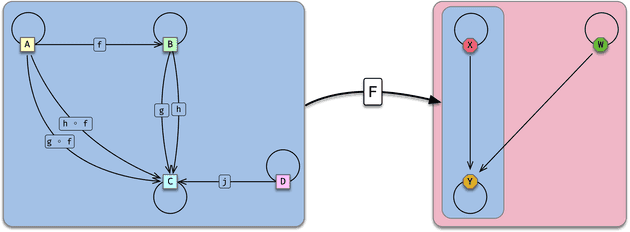
Functors are graph mappings that preserve arrow composition and identities.

If $C$, $D$ are categories, then a (covariant) functor $F$ from $C$ to $D$ is a tuple $(F_0, \mathit{map})$ where

1. $F_0: \mathrm{Ob}(C)\rightarrow \mathrm{Ob}(D)$

(instead of $F_0(X)$ it is common to just write $F_X$).

2. for every pair of objects $X, X'$ in $C$, a function

$$\mathit{map}_{X,X'}: C(X, X')\rightarrow D(F_X, F_{X'})$$

3. $F$ preserves composition

$$F(g f) = F(g) . F(f)$$

4. $F$ preserves identity morphisms

$$F(\mathrm{id}_X) = \mathrm{id}_{F_X}$$

A functor is a data structure that contains a type function F[_] and a regular function map.

Since now there are two categories involved we're going to use Source[_, _] and Target[_, _] for the types of arrows.

trait Functor[
  F[_], Source[_, _], Target[_, _]
](
  using
    S: Category[Source],
    T: Category[Target]
):
  // symbolic aliases
  type ~>[A, B]  = Source[A, B]
  type ~>>[A, B] = Target[A, B]

  def map[A, B](f: A ~> B): F[A] ~>> F[B]
  // helper method to be able to do F(f)
  def apply[A, B](f: A ~> B) = map(f)

  @Law
  def composition[X, Y, Z](f: X ~> Y, g: Y ~> Z) =
    map(g ◦ f) <-> map(g) ◦ map(f)

  @Law
  def identities[X] =
    map(S.id[X]) <-> T.id[F[X]]

On notation

Since Scala 3 supports curried type functions (type lambdas) an alternative alias for functors could be

type -->[From[_, _], To[_, _]] =
  [F[_]] =>> Functor[F, From, To]

To be used like so:

// endofunctors
(C --> C)[F]

// Bifunctor
(C1 × C2 --> D)[F]

// etc

The downside is that it could be hard to keep track of all the different kinds of arrows.

2.1 The identity functor on a category C

type Id[A] = A

object Functor:
  def identity[C[_, _]: Category]: (C --> C) [Id] =
    new Functor { def map[X, Y](f: C[X, Y]) = f }

2.2 Endofunctors

A Functor from a category $C$ to itself.

type Endofunctor[F[_], C[_, _]] = (C --> C) [F]

Later we'll use the following given to create Scala endofunctors from zio.prelude instances.

import zio.prelude.*

given [F[+_]] => (F: classic.Functor[F]) => Endofunctor[F, Scala]:
  def map[A, B](f: A => B) = F.map(f)

// uses classic.Functor[List] to create our Endofunctor instance
summon[Endofunctor[List, Scala]]

2.3 Bifunctors

A bifunctor is a functor whose domain is the product category

type Bifunctor[F[_, _], Prod[_, _], D[_, _]] = 
  Functor[[A] =>> F[_1[A],  _2[A]], Prod, D]

alternatively:

trait Bifunctor2[F[_, _], C1[_, _], C2[_, _], D[_, _]](
    using Category[C1 × C2], Category[D]
  ) extends 
    Functor[[A] =>> F[_1[A],  _2[A]], C1 × C2, D]

2.4 The Hom functor

Given a fixed object $X_0$ in a category $C$, the $\mathrm{Hom}$ functor $C \to \mathbf{Scala}$ sends $A \mapsto \mathrm{Hom}(X_0, A)$.

type Hom[C[_, _], X0] = [A] =>> C[X0, A]

def homFunctor[C[_, _]: Category, X0]: (C --> Scala)[Hom[C, X0]] =
  new Functor:
    def map[A, B](f: C[A, B]): C[X0, A] => C[X0, B] = f ◦ _

2.5 Functor composition

type ⊙[G[_], F[_]] = [A] =>> G[F[A]]

// G ⊙ F
extension [F[_], G[_], C[_, _], D[_, _], E[_, _]] (
  G: (D --> E) [G]) def ⊙ (
  F: (C --> D) [F]
  )(using
    Category[C],
    Category[D],
    Category[E]
  ): (C --> E) [G ⊙ F] =
    new Functor:
      def map[X, Y](f: C[X, Y]) = G(F(f))

3. Natural Transformations

A natural transformation is a family of morphisms between the images of two functors:

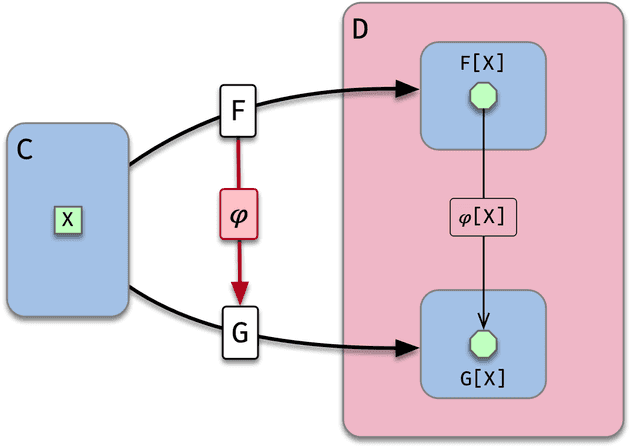
Given two functors $F, G: C \to D$ between the same categories, a natural transformation $\varphi: F \to G$ consists of the following data:

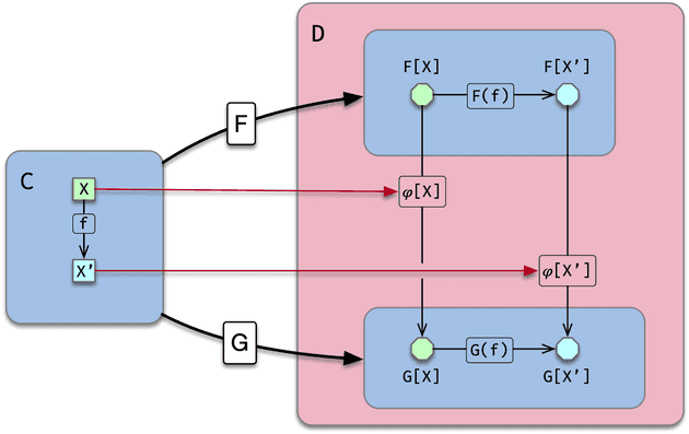
For each object $X$ of $C$ a morphism $\varphi X: FX \to GX$ in $D$ so that, for every arrow $f: X \to X'$ in $C$, we have a commutative square in $D$ (naturality condition of $\varphi$ on $f$)

$$\begin{CD} FX @>{Ff}>> FX' \\ @V{\varphi X}VV @VV{\varphi X'}V \\ GX @>{Gf}>> GX' \end{CD}$$

i.e.

$$\varphi X'.F(f)= G(f). \varphi X$$

trait Nat[From[_], To[_], C[_, _], D[_, _]](
  using
  Category[C],
  Category[D]
) { self =>
  val from: (C --> D) [From]
  val to  : (C --> D) [To]
  
  type ~>[A, B] = D[A, B]

  def apply[X]: From[X] ~> To[X]

  @Law
  def naturality[X, Y](f: C[X, Y]) =
    self[Y] ◦ from(f) <-> to(f) ◦ self[X]
}

One could also define an alias (double fat arrow)

type ==>[F[_], G[_]] =
  [C[_, _], D[_, _]] =>> Nat[F, G, C, D]

and use it like so

(F ==> G)[C, D]

but same caveats apply regarding "way too many arrows" (TM)

3.1 The identity transformation

object Nat:
  def identity[F[_], C[_, _], D[_, _]](
    F: (C --> D)[F]
  )(using
      C: Category[C],
      D: Category[D]): (F ==> F)[C, D] =
    new Nat:
      val from = F
      val to = F
      def apply[X] = D.id[F[X]]

3.2 Vertical composition

Two natural transformations $\varphi: F \to G$ and $\psi: G \to H$ have a vertical composition $\psi\varphi: F \to H$ (also written $\psi.\varphi$)

$$(\psi\varphi)(X)=\psi(X).\varphi(X): FX \to HX$$

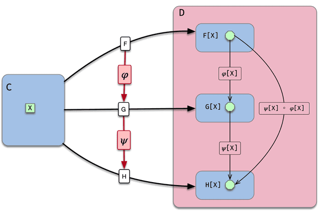
// vertical composition:
// ψ * φ: F ==> H
extension [
    F[_],G[_],H[_], 
    C[_, _], 
    D[_, _]
  ] (ψ: (G ==> H)[C, D]) def * ( 
     φ: (F ==> G)[C, D] )
  (using 
    Category[C], 
    Category[D]): (F ==> H)[C, D]
  =
    new Nat:
      val from = φ.from
      val to   = ψ.to
      def apply[X] = ψ[X] ◦ φ[X] 

3.3 Whisker composition

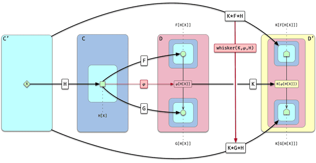
Moreover there is a whisker composition of natural transformations with functors, or reduced horizontal composition, written as $K \varphi H$

$$K \varphi H: K F H \to K G H \\ (K \varphi H)(X) = K(\varphi(H X))$$

// whisker(K, φ, H): K ⊙ F ⊙ H ==> K ⊙ G ⊙ H
def whisker[
  H[_], F[_], G[_], K[_],
  Cp[_, _], C[_, _], 
  D[_, _], Dp[_, _]
](
  K: (D  --> Dp)[K],
  φ: (F  ==> G )[C, D],
  H: (Cp --> C )[H],
)(using
  Category[Cp],
  Category[C],
  Category[D],
  Category[Dp],
): (K ⊙ F ⊙ H ==> K ⊙ G ⊙ H)[Cp, Dp] =
  val F = φ.from
  val G = φ.to
  new Nat:
    val from = K ⊙ F ⊙ H
    val to   = K ⊙ G ⊙ H
    def apply[X] = K(φ[H[X]])

The binary operations $\varphi H$ and $K \varphi$ are also called whisker compositions (obtained by inserting identity functors in the ternary operation)

// (φ *: H): F ⊙ H ==> G ⊙ H
extension [
  H[_], F[_], G[_], 
  Cp[_, _], C[_, _], D[_, _]
](
  φ: (F ==> G)[C, D]) def *: (
  H: (Cp --> C)[H]
)(using
  Category[Cp],
  Category[C],
  Category[D]
): (F ⊙ H ==> G ⊙ H) [Cp, D] =
  whisker(Functor.identity[D], φ, H)
    
// (K :* φ): K ⊙ F ==> K ⊙ G
extension [
  F[_], G[_], K[_], 
  C[_, _], D[_, _], Dp[_, _]
](
  K: (D --> Dp)[K]) def :* (
  φ: (F ==> G)[C, D]
)(using
  Category[C],
  Category[D],
  Category[Dp]
): (K ⊙ F ==> K ⊙ G) [C, Dp] =
  whisker(K, φ, Functor.identity[C])

We've chosen φ *: H and K :* φ to have a visual clue of which side is the natural transformation and which side is the functor.

A natural transformation between two functors in Scala ((F ==> G)[Scala, Scala]) is just a polymorphic function that is capable of transforming one data structure / context into another, without looking at the concrete type argument.

We could say that a functor transforms the contents of a data structure from one type into another:

F[A] => F[B]

whereas a natural transformation performs a structural/context transformation:

F[A] => G[A]

4. Monads

A monad in the category $X$ is a triple $(T, \eta, \mu)$ where $T: X\rightarrow X$ is an endofunctor, while $\eta: 1\rightarrow T$ and $\mu: T^2 \rightarrow T$ are natural transformations (called the unit and multiplication of the monad) which make the following diagrams commute:

$$\begin{CD} T @>{\eta T}>> T^2 @<{T\eta}<< T \\ @| @VV{\mu}V @| \\ T @= T @= T \end{CD}$$

$$\begin{CD} T^3 @>{T\mu}>> T^2 \\ @V{\mu T}VV @VV{\mu}V \\ T^2 @>{\mu}>> T \end{CD}$$

(Grandis, p. 133)

trait Monad[T[_], X[_, _]: Category]:

  // redefine ==> locally (for endofunctors)
  type ==>[H[_], G[_]] = Nat[H, G, X, X]

  def T       : Endofunctor[T, X]
  def pure    : Id ==> T      // 𝜂: 1  ==> T
  def flatten : (T ⊙ T) ==> T // 𝜇: T² ==> T

  @Law
  def unitarity1 =
    (flatten * (pure *: T)) <-> Nat.identity(T)

  @Law
  def unitarity2 =
    (flatten * (T :* pure)) <-> Nat.identity(T)

  @Law
  def associativity =
    flatten * (T :* flatten) <-> flatten * (flatten *: T)

4.1 Monoids in the category of endofunctors

In fact, a monad on the category $X$ is an internal monoid in the category $C = \mathrm{End}(X)$ of endofunctors of $X$ and their natural transformations, equipped with the strict (non-symmetric) monoidal structure given by the composition of endofunctors.

Let's unpack this remark.

4.1.1 Monoidal categories and internal monoids

A (strict) monoidal category $(C, \otimes, E)$ is a category $C$ equipped with a bifunctor

$$\otimes: C \times C \to C$$

that is associative, and an object $E$ called the unit satisfying

$$E \otimes A = A \\ A \otimes E = A \\$$

trait Monoidal[C[_, _]] extends Category[C]:
  type ⨂[_, _]
  type E

  def tensor: Bifunctor[⨂, C × C, C]

  // tensor gives rise to the canonical function
  // f ⨂ g:
  extension [A1, B1, A2, B2]
    ( f: A1 ~> B1) def ⨂ (
      g: A2 ~> B2): (A1 ⨂ A2) ~> (B1 ⨂ B2) =
    tensor[(A1, A2), (B1, B2)]((f, g))

  @Law 
  def unitLeft[A]:
    (E ⨂ A) =:= A

  @Law 
  def unitRight[A]:
    (A ⨂ E) =:= A

  @Law 
  def associativity[A, B, C]:
    (A ⨂ (B ⨂ C)) =:= ((A ⨂ B) ⨂ C)

These three laws are only about objects. A strict monoidal category also needs the same equations for arrows: $1_E \otimes f = f = f \otimes 1_E$ and $(f \otimes g) \otimes h = f \otimes (g \otimes h)$. We leave out those laws.

An internal monoid in $C$ is a triple $(M, e, m)$, consisting of an object $M$ and two arrows $e: E \to M$, $m: M \otimes M \to M$ of $C$, called the unit and multiplication, satisfying:

$$\begin{CD} M @>{e \otimes M}>> M^{\otimes 2} @<{M \otimes e}<< M \\ @| @VV{m}V @| \\ M @= M @= M \end{CD}$$

$$\begin{CD} M^{\otimes 3} @>{M \otimes m}>> M^{\otimes 2} \\ @V{m \otimes M}VV @VV{m}V \\ M^{\otimes 2} @>{m}>> M \end{CD}$$

trait InternalMonoid[C[_, _]](using val C: Monoidal[C]):
  import C.{~>, E, ⨂, id}

  type M
  val e: E ~> M
  val m: M ⨂ M ~> M

  // laws
  @Law
  def unitarity1 =
    C.unitLeft[M].substituteCo[[X] =>> X ~> M](m ◦ (e ⨂ id[M])) <-> id[M]

  @Law
  def unitarity2 =
    C.unitRight[M].substituteCo[[X] =>> X ~> M](m ◦ (id[M] ⨂ e)) <-> id[M]

  @Law
  def associativity =
    m ◦ (m ⨂ id[M]) <->
      C.associativity[M, M, M].substituteCo[[X] =>> X ~> M](m ◦ (id[M] ⨂ m))

For Scala, (E ⨂ M) ~> M and M ~> M are different types, because ⨂ and E are abstract. The laws unitLeft, unitRight and associativity of Monoidal are =:= values. substituteCo uses such a value to change the type of one side. Thus the two sides of each law have the same type.

4.1.2 The category of endofunctors and natural transformations

In order to describe this category we'll need a higher order version of CategoryTC (that we used to create the category of groups).

// A category of type functions with some constraint P
trait CategoryTC1[P[F[_]], Hom[F[_], G[_]]]:

  type ~>[F[_], G[_]] = Hom[F, G]

  def id[F[_]](using P[F]): F ~> F

  extension [F[_]: P, G[_]: P, H[_]: P] 
    (m: G ~> H) def ◦ (n: F ~> G): F ~> H

This means objects will be type functions $\mathbb{T} \to \mathbb{T}$ with some constraint represented by P[_[_]] and Hom is a function $(\mathbb{T} \to \mathbb{T}, \mathbb{T} \to \mathbb{T}) \to \mathbb{T}$.

// Given a Category[X] creates the category whose objects are 
// endofunctors of X and whose morphisms are the natural 
// transformations between them.

def endo[X[_, _]: Category] =

  type Hom[H[_], G[_]] = (H ==> G)[X, X]
  
  type EndoX[F[_]] = Endofunctor[F, X]

  new CategoryTC1[EndoX, Hom]:

    def id[F[_]](using f: EndoX[F]): F ~> F =
      Nat.identity(f)

    extension [F[_]: EndoX, G[_]: EndoX, H[_]: EndoX] 
      (m: G ~> H) def ◦ (n: F ~> G): F ~> H =
      m * n

For example, this is the identity natural transformation for List in the category of endofunctors in Scala:

endo[Scala].id[List]

And this is the category of endofunctors for the Kleisli category of functions A => Option[B]:

// a minimal Kleisli arrow and its category
final case class Kleisli[F[_], A, B](run: A => F[B])

given Category[[A, B] =>> Kleisli[Option, A, B]]:
  def id[A] = Kleisli(Some(_))
  extension [A, B, C] (g: Kleisli[Option, B, C])
    def ◦ (f: Kleisli[Option, A, B]) = Kleisli((a: A) => f.run(a).flatMap(g.run))

val optionKleisliEndo = endo[[A, B] =>> Kleisli[Option, A, B]]

4.1.3 Monoids in the category of endofunctors

In fact, a monad on the category $X$ is an internal monoid in the category $C = \mathrm{End}(X)$ of endofunctors of $X$ and their natural transformations, equipped with the strict monoidal structure given by the composition of endofunctors.

Below is a direct encoding of the monoidal structure on endofunctors using CategoryTC1, plus the corresponding internal monoid. Its unit and associativity laws are equalities of type functions. =:= is only for proper types, so we use =~=, a small equality of type functions with the same substituteCo:

import scala.compiletime.deferred

// F =~= G: the type functions F and G are equal (=:= is only for proper types)
trait =~=[F[_], G[_]]:
  def substituteCo[H[_[_]]](h: H[F]): H[G]

def refl[F[_]]: F =~= F =
  new =~=[F, F]:
    def substituteCo[H[_[_]]](h: H[F]) = h

trait MonoidalTC1[P[F[_]], Hom[F[_], G[_]]] extends CategoryTC1[P, Hom]:
  type ⨂[F[_], G[_]] <: [A] =>> Any
  type E[_]

  // E and F ⨂ G are objects of the category too
  given unitObj: P[E] = deferred
  given tensorObj: [F[_]: P, G[_]: P] => P[F ⨂ G] = deferred

  def tensor[F[_]: P, G[_]: P, H[_]: P, I[_]: P](
    f: F ~> H,
    g: G ~> I
  ): (F ⨂ G) ~> (H ⨂ I)

  // tensor gives rise to the canonical function
  // f ⨂ g:
  extension [F[_]: P, G[_]: P, H[_]: P, I[_]: P]
    (f: F ~> H) def ⨂ (g: G ~> I): (F ⨂ G) ~> (H ⨂ I) =
    tensor(f, g)

  @Law
  def unitLeft[F[_]]:
    (E ⨂ F) =~= F

  @Law
  def unitRight[F[_]]:
    (F ⨂ E) =~= F

  @Law
  def associativity[F[_], G[_], H[_]]:
    (F ⨂ (G ⨂ H)) =~= ((F ⨂ G) ⨂ H)

trait InternalMonoid1[P[F[_]], Hom[F[_], G[_]]]:
  val C: MonoidalTC1[P, Hom]
  import C.{~>, E, ⨂, ◦, id, given}

  type M[_]
  given P[M] = deferred
  val e: E ~> M
  val m: (M ⨂ M) ~> M

  // laws omitted (same shape as InternalMonoid)

def endoMonoidal[X[_, _]: Category] =
  type Hom[F[_], G[_]] = (F ==> G)[X, X]
  type EndoX[F[_]] = Endofunctor[F, X]

  new MonoidalTC1[EndoX, Hom]:
    def id[F[_]](using f: EndoX[F]): F ~> F =
      Nat.identity(f)

    extension [F[_]: EndoX, G[_]: EndoX, H[_]: EndoX]
      (m: G ~> H) def ◦ (n: F ~> G): F ~> H =
      m * n

    type ⨂[F[_], G[_]] = F ⊙ G
    type E[A] = A // identity endofunctor

    override given unitObj: EndoX[E] = Functor.identity[X]
    override given tensorObj: [F[_]: EndoX as F, G[_]: EndoX as G] => EndoX[F ⨂ G] = F ⊙ G

    def unitLeft[F[_]]: (E ⨂ F) =~= F = refl
    def unitRight[F[_]]: (F ⨂ E) =~= F = refl
    def associativity[F[_], G[_], H[_]]: (F ⨂ (G ⨂ H)) =~= ((F ⨂ G) ⨂ H) = refl

    def tensor[F[_]: EndoX, G[_]: EndoX as G, H[_]: EndoX as H, I[_]: EndoX](
      α: F ~> H,
      β: G ~> I
    ): (F ⨂ G) ~> (H ⨂ I) =
      (H :* β) * (α *: G)

We can now write a monad-like structure directly in terms of MonoidalTC1:

trait MonadTC1[P[F[_]], Hom[F[_], G[_]]]:
  val C: MonoidalTC1[P, Hom]
  import C.{~>, E, ⨂, ◦, id, given}

  type T[_]
  given P[T] = deferred

  def pure    : E ~> T
  def flatten : (T ⨂ T) ~> T

  @Law
  def unitarity1 =
    C.unitLeft[T].substituteCo[[F[_]] =>> F ~> T](flatten ◦ (pure ⨂ id[T])) <-> id[T]

  @Law
  def unitarity2 =
    C.unitRight[T].substituteCo[[F[_]] =>> F ~> T](flatten ◦ (id[T] ⨂ pure)) <-> id[T]

  @Law
  def associativity =
    flatten ◦ (flatten ⨂ id[T]) <->
      C.associativity[T, T, T].substituteCo[[F[_]] =>> F ~> T](flatten ◦ (id[T] ⨂ flatten))

In the monoidal category of endofunctors, E ≙ Id and ⨂ ≙ ⊙, so this specializes to the usual notion of a monad. We can describe the correspondence explicitly:

type EndoMonoidal[X[_, _]] =
  MonoidalTC1[
    [F[_]] =>> Endofunctor[F, X],
    [F[_], G[_]] =>> (F ==> G)[X, X]
  ]

def monadToInternal[X[_, _]: Category](M: MonadTC1[
  [F[_]] =>> Endofunctor[F, X],
  [F[_], G[_]] =>> (F ==> G)[X, X]
]) =
  import M.given
  new InternalMonoid1[
    [F[_]] =>> Endofunctor[F, X],
    [F[_], G[_]] =>> (F ==> G)[X, X]
  ]:
    val C: M.C.type = M.C
    type M = M.T
    val e = M.pure
    val m = M.flatten

def internalToMonad[X[_, _]: Category](M: InternalMonoid1[
  [F[_]] =>> Endofunctor[F, X],
  [F[_], G[_]] =>> (F ==> G)[X, X]
]) =
  import M.given
  new MonadTC1[
    [F[_]] =>> Endofunctor[F, X],
    [F[_], G[_]] =>> (F ==> G)[X, X]
  ]:
    val C: M.C.type = M.C
    type T = M.M
    def pure    = M.e
    def flatten = M.m

These two mappings are inverse on the structure fields.

With these definitions in place, compare the structure of InternalMonoid1, MonadTC1, and Monad.

trait InternalMonoid1[P[F[_]], Hom[F[_], G[_]]]:
  val C: MonoidalTC1[P, Hom]
  import C.{~>, E, ⨂, ◦, id, given}
  //
  //
  type M[_]
  given P[M] = deferred
  val e: E ~> M
  val m: (M ⨂ M) ~> M

trait MonadTC1[P[F[_]], Hom[F[_], G[_]]]:
  val C: MonoidalTC1[P, Hom]
  import C.{~>, E, ⨂, ◦, id, given}
  //
  //
  type T[_]
  given P[T] = deferred
  def pure    : E ~> T
  def flatten : (T ⨂ T) ~> T

trait Monad[T[_], X[_, _]]
  (using Category[X]):
  type ==>[F[_], G[_]] = 
    Nat[F, G, X, X]
  //
  //
  def T       : Endofunctor[T, X]
  def pure    : Id ==> T
  def flatten : (T ⊙ T) ==> T

C.unitLeft[M]
  .substituteCo[[F[_]] =>> F ~> M](
    m ◦ (e ⨂ id[M])) <-> id[M]

C.unitLeft[T]
  .substituteCo[[F[_]] =>> F ~> T](
    flatten ◦ (pure ⨂ id[T])) <-> id[T]

(flatten * (pure *: T)) <-> Nat.identity(T)

C.unitRight[M]
  .substituteCo[[F[_]] =>> F ~> M](
    m ◦ (id[M] ⨂ e)) <-> id[M]

C.unitRight[T]
  .substituteCo[[F[_]] =>> F ~> T](
    flatten ◦ (id[T] ⨂ pure)) <-> id[T]

(flatten * (T :* pure)) <-> Nat.identity(T)

m ◦ (m ⨂ id[M]) <->
C.associativity[M, M, M]
  .substituteCo[[F[_]] =>> F ~> M](
    m ◦ (id[M] ⨂ m))

flatten ◦ (flatten ⨂ id[T]) <->
C.associativity[T, T, T]
  .substituteCo[[F[_]] =>> F ~> T](
    flatten ◦ (id[T] ⨂ flatten))

flatten * (flatten *: T) <-> 
flatten * (T :* flatten)

4.2 Monads in Scala

If we set the category to be Scala (of types and functions) several things happen:

• Endofunctor becomes the usual classic.Functor

• Natural transformations become:

trait Nat[F[+_]: classic.Functor, G[+_]: classic.Functor]:
  def apply[A]: F[A] => G[A]

• Our specialized monad becomes:

trait Monad[T[+_]: classic.Functor]:
  def pure   : Nat[Id,  T]
  def flatten: Nat[T ⊙ T, T]

• Simplifying even more by inlining the apply method of both transformations:

import zio.prelude.*

trait Monad[T[+_]: classic.Functor]:
  def pure   [A]:     A   => T[A] 
  def flatten[A]: T[T[A]] => T[A]

  def flatMap[A, B](a: T[A])(f: A => T[B]): T[B] =
    flatten(Covariant[T].map(f)(a))

voila!

5. The Yoneda lemma

Let $F, G:C\rightarrow \mathbf{Set}$ be two functors, with $F=C(X_0, \_)$. The canonical mapping

$$\begin{matrix} y: & \mathrm{Nat}(F,G) & \rightarrow & G_{X_0} \\ & \varphi & \mapsto & \varphi_{X_0}(\mathrm{id}_{X_0}) \end{matrix}$$

from the set of natural transformations $\varphi:F \rightarrow G$ to the set $G(X_0)$ is a bijection.

The inverse mapping is given by

$$\begin{matrix} y': & G_{X_0} & \rightarrow & \mathrm{Nat}(\mathrm{Hom}(X_0,\_),G) \\ & z & \mapsto & y'(z)_X f:=G_f(z) \ \ \forall X \\ & & & _{f: C(X_0, X)} \end{matrix}$$

(Grandis, p. 44)

A bijection between two types A and B can be naturally expressed as an instance of the following type

case class Bijection[A, B](
  from: A => B,
  to  : B => A
):
  // satisfying laws
  @Law
  def IdB = (from ◦ to) <-> identity[B]

  @Law
  def IdA = (to ◦ from) <-> identity[A]

type ≅[A, B] = Bijection[A, B]

Since our base category is Scala (instead of Set) then both $F, G$ will be functors from $C$ to Scala.

def yonedaLemma[C[_, _], G[_], X0](G: (C --> Scala)[G])
  (using C: Category[C] ) =
  import C.id

  val F: (C --> Scala)[Hom[C, X0]] = homFunctor[C, X0]

  // at this point we know that F, G are functors 
  // and C is a category, so we can simplify a bit 
  // by working with the natural transformation as a 
  // polymorphic function instead of the wrapper type Nat:
  type ==>[F[_], G[_]] = 
    [X] => F[X] => G[X]
  // NOTE: We still assume any φ: F ==> G is natural.

  // ----------------
  // The Yoneda lemma
  // ----------------

  // the canonical mapping:
  val y : (Hom[C, X0] ==> G) => G[X0] =
                     φ     => φ[X0]( id[X0] )

  // is a bijection with inverse:
  val yp: G[X0] => (Hom[C, X0] ==> G) =
            z   =>   ([X]    => (f: C[X0, X]) => G(f)(z))
    
  // i.e.
  // y  ◦ yp <-> identity[G[X0]]
  // yp ◦ y  <-> identity[Hom[C, X0] ==> G]

  // Or more concisely:
  val yoneda: (Hom[C, X0] ==> G) ≅ G[X0] =
    Bijection(y, yp)

Proof:

  // Assumptions used below:
  // - φ is natural.
  // - G preserves identities and composition (functor laws).
  // - For F = homFunctor, F(f)(id[X0]) = f (right identity, identityR).
  // a) yp(y(𝜑)) == 𝜑
  def proofPart1(φ: Hom[C, X0] ==> G) =

    // by definition of y:
    yp(y(φ)) == yp( φ[X0] { id[X0] } )

    // by definition of yp:
    yp(y(φ)) == ( [X] => (f: C[X0, X]) => G(f) { φ[X0] { id[X0] } } )

    // which in Scala is the same as:
    yp(y(φ)) == ( [X] => (f: C[X0, X]) => (G(f) ◦ φ[X0]) { id[X0] } )

    // by the naturality condition: G(f) ◦ φ[X0] === φ[X] ◦ F(f)
    yp(y(φ)) == ( [X] => (f: C[X0, X]) => (φ[X] ◦ F(f)) { id[X0] } )

    yp(y(φ)) == ( [X] => (f: C[X0, X]) => φ[X] { F(f) { id[X0] } } )

    // by definition of homFunctor: F(f)( id[X0] ) == f ◦ id[X0]
    // and by the right identity law (identityR) of C: f ◦ id[X0] == f
    yp(y(φ)) == ( [X] => (f: C[X0, X]) => φ[X] { f } )
    
    // applying eta reduction two times:
    // yp(y(φ)) == ( [X] => φ[X]  ) == φ
    
    yp(y(φ)) == φ


  // b) y(yp(z)) == z
  def proofPart2(z: G[X0]) =

    // by definition of yp:
    y(yp(z)) == y( [X] => (f: C[X0, X]) => G(f)(z) )

    // by definition of y:
    y(yp(z)) == ( [X] => (f: C[X0, X]) => G(f)(z) ) { id[X0] }
    
    // evaluating the right hand side
    y(yp(z)) == G(id[X0])(z)

    // Since G maps identities to identities:
    // G(id[X0]) == Scala.id[G[X0]] == identity[G[X0]] == (x => x)
    y(yp(z)) == z     

  // c) yp(z) is natural, so yp(z) is really in Nat(F, G):
  //    for g: C[X, Y], yp(z)[Y] ◦ F(g) == G(g) ◦ yp(z)[X]
  def proofPart3[X, Y](z: G[X0], g: C[X, Y], f: C[X0, X]) =

    // by definition of homFunctor: F(g)(f) == g ◦ f
    (yp(z)[Y] ◦ F(g))(f) == yp(z)[Y](g ◦ f)

    // by definition of yp:
    (yp(z)[Y] ◦ F(g))(f) == G(g ◦ f)(z)

    // G preserves composition (functor law):
    (yp(z)[Y] ◦ F(g))(f) == (G(g) ◦ G(f))(z)

    // by definition of yp:
    (yp(z)[Y] ◦ F(g))(f) == (G(g) ◦ yp(z)[X])(f)

    // This holds for every f, so yp(z)[Y] ◦ F(g) == G(g) ◦ yp(z)[X]

// Q.E.D

This is pretty much what one would write on paper, except that it is more verbose. The other difference is that the compiler will help us ensure that expressions at least typecheck.

6. Bibliography

• M. Grandis, Category Theory and Applications: A Textbook for Beginners, first edition, World Scientific, 2018.
• F. W. Lawvere and S. H. Schanuel, Conceptual Mathematics: A First Introduction to Categories, Cambridge University Press, 2nd edition, 2009.
• Scala 3 documentation: https://docs.scala-lang.org/.

7. Changelog

• Jun 29, 2022: Code repository added.
• Feb 5, 2026: Scala 3 version 3.8.
• Sep 24, 2026: Scala 3 version 3.9. The code uses the current Scala 3 syntax, and the two sides of each law have the same type.